LAMP for Survival Analysis
Survival LAMP is an extended version of LAMP (Terada et al 2013) for performing multiple testing correction in finding combinatorial markers using log-rank test in survival analysis. Details and usage of the original LAMP can be found here.
How to run LAMP for survival analysis:
- Clone or download from GitHub.
- Compile: run
makein corresponding directory - Run:
python lampSA.py -p logrank [item_file] [status_file] [significance_level] -t [time_file] > [output_file]EXAMPLE:
python lampSA.py -p logrank sample/sample_logrank_item.csv sample/sample_logrank_status.csv 0.05 -t sample/sample_logrank_time.csv > sample/sample_logrank_output.txt
Input Files:
- ITEM FILE
- similar format to the original LAMP item file, this file contains association information of samples/individuals and markers
- first row as header (commented first entry, contains marker identifiers)
- first column contains the list of sample/individual IDs (one sample/individual per row)
- succeeding columns represent markers (e.g. gene, SNPs, etc.) (one marker per column)
- entries are 1 or 0 (integer type)
- file format: csv
- example: sample/sample_logrank_item.csv
- STATUS FILE
- similar format to the original LAMP value file, except that it contains the status of samples/individuals
- first row as header (commented first entry similar to item file)
- first column must be the same as the item file
- second column contains status of corresponding samples/individuals (1 = event, 0 = censored)
- file format: csv
- example: sample/sample_logrank_status.csv
- TIME FILE
- contains survival time information of samples/individuals
- first row as header (commented first entry similar to item and status files)
- first column must be the same as the item and value files
- second column contains survival time of corresponding samples/individuals (e.g. in months, years, or days)
- file format: csv
- example: sample/sample_logrank_time.csv
Output File:
- similar format to the original LAMP output file
- example: sample/sample_logrank_output.txt
# Survival LAMP ver. 1.0 # item-file: sample/sample_logrank_item.csv # value-file: sample/sample_logrank_status.csv # time-file: sample/sample_logrank_time.csv # significance-level: 0.05 # P-value computing procedure: logrank # # of tested elements: 9, # of samples: 292, # of positive samples: 101 # Adjusted significance level: 0.0005618, Correction factor: 89 (# of target rows >= 1) # # of significant combinations: 5 Rank Raw p-value Adjusted p-value Combination Arity # of target rows # of failed targets 1 1.738e-05 0.0015468 r60_n9,G3PDH_570 2 14 10 2 2.4931e-05 0.0022188 r60_n9,G3PDH_570,r60_1,r60_3 4 9 7 3 8.6793e-05 0.0077246 r60_n9,G3PDH_570,r60_3 3 11 8 4 0.00039433 0.035096 r60_n9,r60_a22,G3PDH_570 3 10 7 5 0.00042816 0.038106 r60_n9,Pro25G,G3PDH_570 3 10 7 Time (sec.): Computing correction factor 0.620, P-value 1.363, Total 1.983 - # of tested elements = number of marker columns in item file
- # of samples = number of samples/individuals included (not counting censored samples/individuals after first failure time)
- # of positive samples = number of failed samples/individuals (i.e. status = 1)
- # of target rows = number of samples/individuals affected by the combination
- # of failed targets = number of samples/individuals affected by the combination whose status is 1 (i.e. failures)
Log-rank Test and Kaplan-Meier Curves in R
Performing log-rank test and generating KM plots for the combination results can be implemented using the survival package in R:
Log-rank Test
library(survival)

# read the three input files for LAMP
df = read.table("sample/sample_logrank_item.csv", sep = ",", header = T, comment.char = "", check.names = F, stringsAsFactors = F)
df_status = read.table("sample/sample_logrank_status.csv", sep = ",", header = T, comment.char = "", check.names = F, stringsAsFactors = F)
df_time = read.table("sample/sample_logrank_time.csv", sep = ",", header = T, comment.char = "", check.names = F, stringsAsFactors = F)

# can join into one data frame, otherwise use respective columns of each data frame separately
df$TIME = df_time$TIMErecurrence; df$STATUS = df_status$EVENTrecurrence

# compute for combination value by getting the product for each sample/individual, add to data frame as column 'COMB'
# example for combination r60_n9,G3PDH_570
df$COMB = apply(df[,c("r60_n9","G3PDH_570")], 1, prod)

# perform log-rank test
lr = survdiff(Surv(TIME, STATUS) ~ COMB, data = df)
print(lr)

Call:
survdiff(formula = Surv(TIME, STATUS) ~ COMB, data = df)

         N Observed Expected (O-E)^2/E (O-E)^2/V
COMB=0 281       91    98.14      0.52      18.5
COMB=1  14       10     2.86     17.87      18.5

 Chisq= 18.5  on 1 degrees of freedom, p= 1.74e-05
In the R results:
- COMB=0: population not containing the corresponding marker combination (i.e. item file value = 0 for at least one of the markers)
- COMB=1: population containing the corresponding marker combination (i.e. item file value = 1 for all of the markers)
- N >= # of target rows in the LAMP results (since LAMP disregards censored samples before first failure time. However, this has no effect on the resulting p-value)
- Observed = # of failed targets in the LAMP results
- p = raw log-rank p-value of the combination
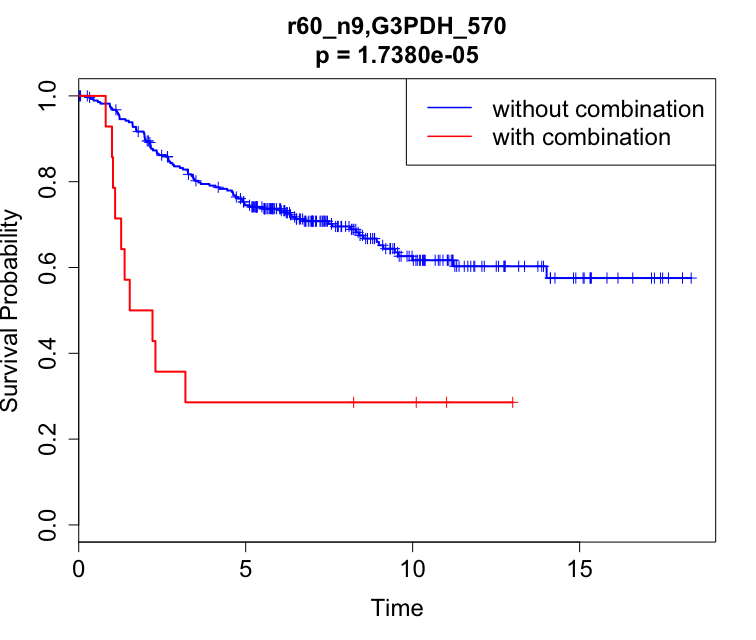
Plotting KM Curves
# fit Kaplan-Meier and plot curves
fit = survfit(Surv(TIME, STATUS) ~ COMB, data = df)
plot(fit)

# add tick marks for censored data and color legends
plot(fit, mark.time = T, col = c("blue", "red"), xlab = "Time", ylab = "Survival Probability", lwd = 2, lty = 1, cex.lab = 1.5, cex.axis = 1.5, cex.main = 1.5, cex.sub = 1.5)
legend("topright", c("without combination", "with combination"), lty = 1, col = c("blue","red"), lwd = 1.5, cex = 1.5)

# getting p-value from log-rank test result
pval = 1 - pchisq(lr$chisq, 1)
title(sprintf("r60_n9,G3PDH_570\np = %.4e", pval), cex.main = 1.5)
The code above will produce the following plot: